I am going to be going in depth and looking at the worst games in college football from the 2019 season.
First I need to load the correct library, tidyverse, and then load my data in, all of the games from the 2019 college football season.
library(tidyverse)

badlogs <- read_csv("~/Desktop/SPMC 350 Files/homework/data/badfootballlogs19.csv")
First, I need to fix the Result column. Currently, its data is in W/L format and I want separate columns called Outcome and Score using the separate command.
badlogs %>%
  separate(Result, into=c("Outcome", "Score"), sep=" ")
## # A tibble: 1,662 × 52
## Game Date HomeAway Opponent Outcome Score PassingCmp PassingAtt PassingPct
## <dbl> <chr> <chr> <chr> <chr> <chr> <dbl> <dbl> <dbl>
## 1 1 8/24/… N Miami (… W (24-… 17 27 63
## 2 2 9/7/19 <NA> Tenness… W (45-… 30 36 83.3
## 3 3 9/14/… @ Kentucky W (29-… 21 30 70
## 4 4 9/21/… <NA> Tenness… W (34-… 24 34 70.6
## 5 5 9/28/… <NA> Towson W (38-… 24 28 85.7
## 6 6 10/5/… <NA> Auburn W (24-… 25 39 64.1
## 7 7 10/12… @ Louisia… L (28-… 24 44 54.5
## 8 8 10/19… @ South C… W (38-… 21 33 63.6
## 9 9 11/2/… N Georgia L (17-… 21 33 63.6
## 10 10 11/9/… <NA> Vanderb… W (56-… 27 40 67.5
## # … with 1,652 more rows, and 43 more variables: PassingYds <dbl>,
## # PassingTD <dbl>, RushingAtt <dbl>, RushingYds <dbl>, RushingAvg <dbl>,
## # RushingTD <dbl>, OffensivePlays <dbl>, OffensiveYards <dbl>,
## # OffenseAvg <dbl>, FirstDownPass <dbl>, FirstDownRush <dbl>,
## # FirstDownPen <dbl>, FirstDownTotal <dbl>, Penalties <dbl>,
## # PenaltyYds <dbl>, Fumbles <dbl>, Interceptions <dbl>, TotalTurnovers <dbl>,
## # TeamFull <chr>, TeamURL <chr>, DefPassingCmp <dbl>, DefPassingAtt <dbl>, …Now that I have the Result column separated out into Outcome and Score, I want to get rid of the parentheses that surround the scores. This is where I’ll use the gsub command.
badlogs %>%
  separate(Result, into=c("Outcome", "Score"), sep=" ") %>%
  mutate(Score = gsub(")", "", Score, fixed = TRUE)) %>%
  mutate(Score = gsub("(", "", Score, fixed = TRUE))
## # A tibble: 1,662 × 52
## Game Date HomeAway Opponent Outcome Score PassingCmp PassingAtt PassingPct
## <dbl> <chr> <chr> <chr> <chr> <chr> <dbl> <dbl> <dbl>
## 1 1 8/24/… N Miami (… W 24-20 17 27 63
## 2 2 9/7/19 <NA> Tenness… W 45-0 30 36 83.3
## 3 3 9/14/… @ Kentucky W 29-21 21 30 70
## 4 4 9/21/… <NA> Tenness… W 34-3 24 34 70.6
## 5 5 9/28/… <NA> Towson W 38-0 24 28 85.7
## 6 6 10/5/… <NA> Auburn W 24-13 25 39 64.1
## 7 7 10/12… @ Louisia… L 28-42 24 44 54.5
## 8 8 10/19… @ South C… W 38-27 21 33 63.6
## 9 9 11/2/… N Georgia L 17-24 21 33 63.6
## 10 10 11/9/… <NA> Vanderb… W 56-0 27 40 67.5
## # … with 1,652 more rows, and 43 more variables: PassingYds <dbl>,
## # PassingTD <dbl>, RushingAtt <dbl>, RushingYds <dbl>, RushingAvg <dbl>,
## # RushingTD <dbl>, OffensivePlays <dbl>, OffensiveYards <dbl>,
## # OffenseAvg <dbl>, FirstDownPass <dbl>, FirstDownRush <dbl>,
## # FirstDownPen <dbl>, FirstDownTotal <dbl>, Penalties <dbl>,
## # PenaltyYds <dbl>, Fumbles <dbl>, Interceptions <dbl>, TotalTurnovers <dbl>,
## # TeamFull <chr>, TeamURL <chr>, DefPassingCmp <dbl>, DefPassingAtt <dbl>, …Looks good. Now, I want to separate the Score column into two columns named TeamScore and OpponentScore. This is also used with the separate command. After that, I need to mutate the TeamScore and OpponentScore into numerical values. I’ll rename this dataframe to notsobadlogs.
badlogs %>%
  separate(Result, into=c("Outcome", "Score"), sep=" ") %>%
  mutate(Score = gsub(")", "", Score, fixed = TRUE)) %>%
  mutate(Score = gsub("(", "", Score, fixed = TRUE)) %>%
  separate(Score, into=c("TeamScore", "OpponentScore"), sep="-") %>%   mutate(TeamScore = as.numeric(TeamScore), OpponentScore = as.numeric(OpponentScore)) -> notsobadlogs
Now, for the exciting part, I’m going to look at the worst games in college football. I need to mutate a new field called Differential. This field is taking TeamScore - OpponentScore.
notsobadlogs %>%
  mutate(Differential = TeamScore - OpponentScore) -> notsobadlogs
Next, I’m creating a dataframe called worstgames where the differential is greater than 65 points.
worstgames <- notsobadlogs %>%
  filter(Differential > 65)
Finally let’s create a scatter plot showcasing the worst games with TeamScore on the X axis and OpponentScore on the Y axis. I’m going to add our worstgames data frame in red.
ggplot() + geom_point(data = notsobadlogs, aes(x = TeamScore, y = OpponentScore), color = "grey") +
  geom_point(data = worstgames, aes(x = TeamScore, y = OpponentScore), color = "red")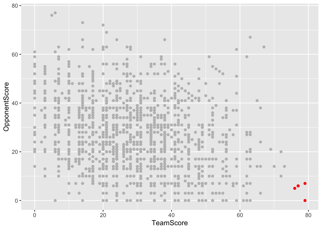
To circle our worstgames, I need the library called “ggalt.” After that, I’ll use the code geom_encircle.
library(ggalt)ggplot() + geom_point(data = notsobadlogs, aes(x = TeamScore, y = OpponentScore), color = "grey") +
geom_point(data = worstgames, aes(x = TeamScore, y = OpponentScore), color = "red") +
geom_encircle(data = worstgames, aes(x = TeamScore, y = OpponentScore), s_shape=0.1, expand=0.045, colour="black")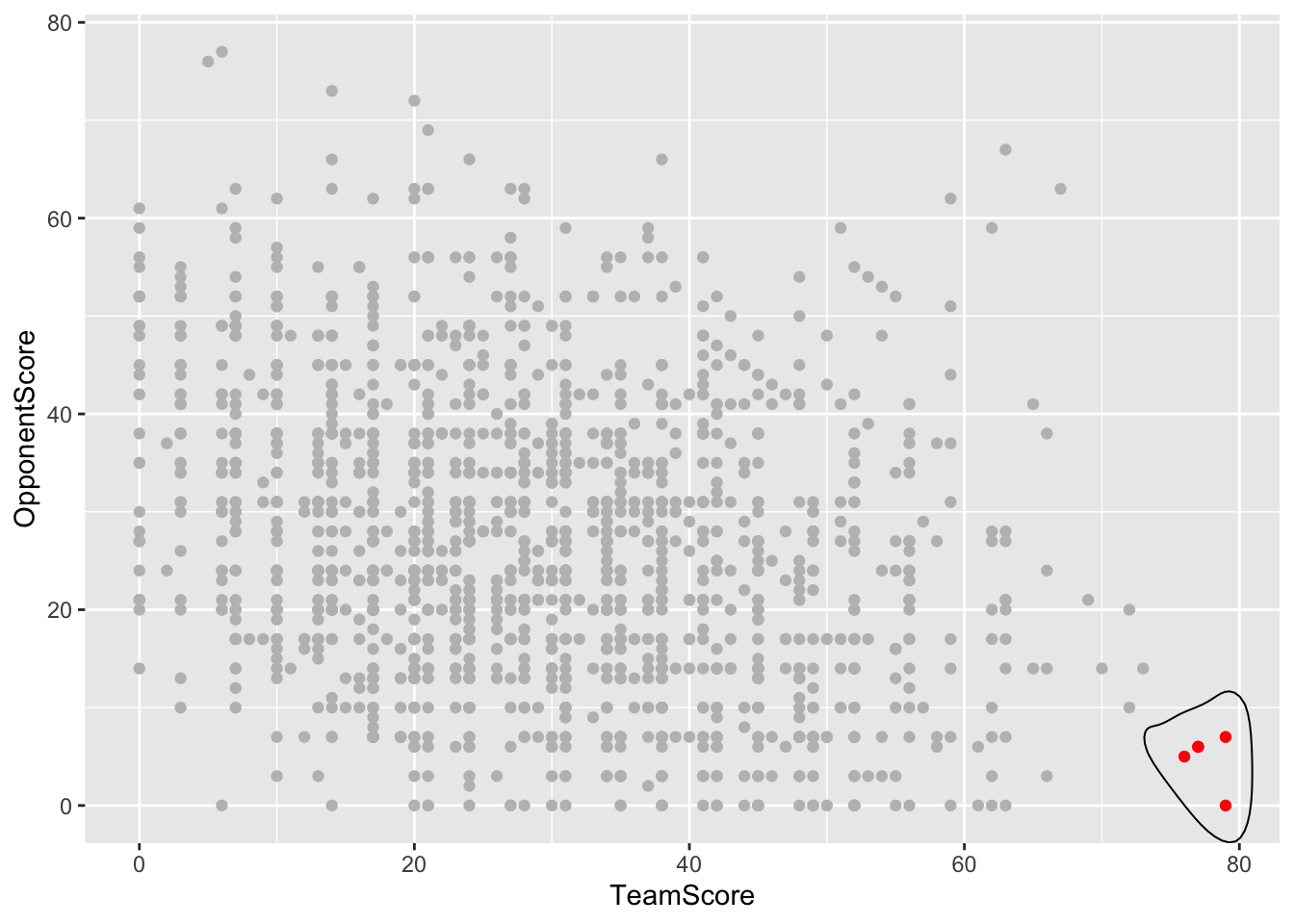
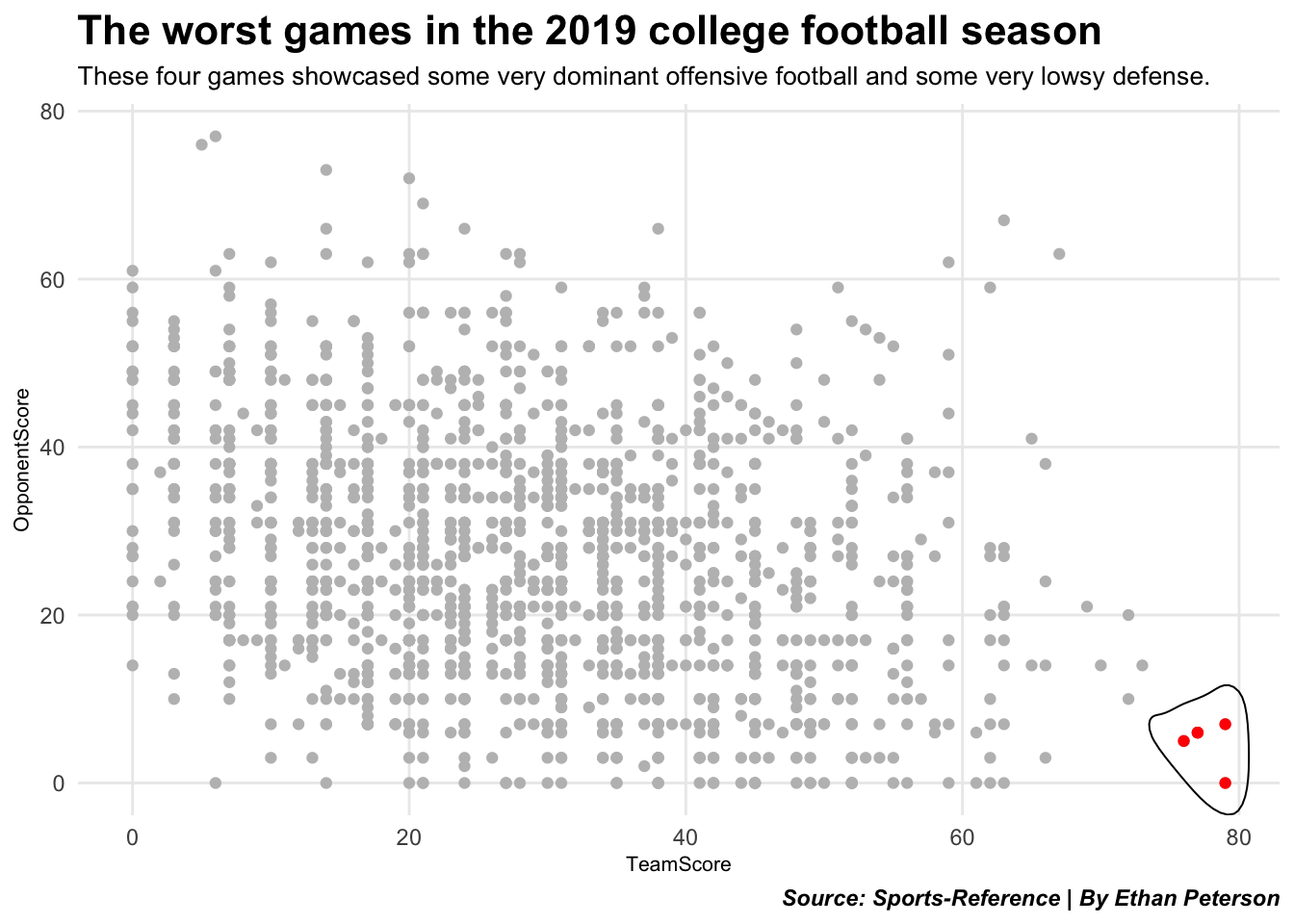
Now, lets add a title, subtitle, labels, a caption, and other small details to make this chart pop.
ggplot() + geom_point(data = notsobadlogs, aes(x = TeamScore, y = OpponentScore), color = "grey") +
  geom_point(data = worstgames, aes(x = TeamScore, y = OpponentScore), color = "red") +
geom_encircle(data = worstgames, aes(x = TeamScore, y = OpponentScore), s_shape=0.1, expand=0.045, colour="black") +
labs(title="The worst games in the 2019 college football season", subtitle="These four games showcased some very dominant offensive football and some very lowsy defense.", caption="Source: Sports-Reference | By Ethan Peterson") +
theme_minimal() +
theme(
plot.title = element_text(size = 16, face = "bold"),
axis.title = element_text(size = 8),
plot.subtitle = element_text(size=10),
plot.caption = element_text(face = "bold.italic"),
panel.grid.minor = element_blank()
)